Background
Basketball has been my favorite sport of all time for as long as I can remember. I started playing back in secondary school and while I do not play as much these days, I still follow the news and watch the NBA games. We all know that Stephen Curry is one of the greatest three-point shooters in NBA history so I pulled some data and saw the three-points made percentages for the 2023-24 season, I expected his name on the top. Instead, the highest percentage in the league belonged to... Luke Kornet?! A centre, sitting at a perfect 100%? As it turns out, Kornet had taken exactly 1 attempt the entire season and made it. A perfect percentage built on a sample size of one.
That's what sparked today's topic, could I use empirical Bayes shrinkage to build a fairer and more reliable way to rank shooters?
Getting the data
#| echo: false
library(hoopR)
library(dplyr)
library(tidyverse)
We can obtain the NBA basketball data using the R package called hoopR and we can specify year or multiple years to pull the data. For 2023-24 season, the data contains 57 variables and 35028 observations. Each row appears to represent an individual player’s statistics for a particular game, meaning that the same player appears many times across the dataset.
# Single season (2024 = the 2023-24 season)
player_box = load_nba_player_box(seasons = 2024)
head(player_box)
# A tibble: 6 × 57
    game_id season season_type game_date  game_date_time      athlete_id
      <int>  <int>       <int> <date>     <dttm>                   <int>
1 401656363   2024           3 2024-06-17 2024-06-17 20:30:00    4278078
2 401656363   2024           3 2024-06-17 2024-06-17 20:30:00    3936099
3 401656363   2024           3 2024-06-17 2024-06-17 20:30:00    4278049
4 401656363   2024           3 2024-06-17 2024-06-17 20:30:00       6442
5 401656363   2024           3 2024-06-17 2024-06-17 20:30:00    3945274
6 401656363   2024           3 2024-06-17 2024-06-17 20:30:00    2960236
# ℹ 51 more variables
Since we want to look at the total three-points made and attempts for the entire season, we need to process the data and group by for every player in 2024. As mentioned at the start, Kornet is ranked at the top with 100%.
# Filter out to obtain three points attempts for each player
# Data seem to be displayed for every single game
three_pts_2024 = player_box %>%
  dplyr::select(season,season_type, athlete_id, athlete_display_name,
         three_point_field_goals_made,three_point_field_goals_attempted) %>%
  group_by(season, athlete_id, athlete_display_name) %>%
  summarise(three_point_field_goals_made = sum(three_point_field_goals_made, na.rm = TRUE),
            three_point_field_goals_attempted = sum(three_point_field_goals_attempted, na.rm = TRUE),
            .groups = "drop") %>%
  mutate(three_point_pct = three_point_field_goals_made/three_point_field_goals_attempted,
         three_point_pct = ifelse(is.nan(three_point_pct), 0, three_point_pct)) %>%
  arrange(desc(three_point_pct))


head(three_pts_2024)
# A tibble: 6 × 6
  season athlete_display_name three_point_field_goals_made three_point_field_goals_attempted three_point_pct
   <int> <chr>                                       <int>                             <int>           <dbl>
1   2024 Luke Kornet                                     1                                 1               1
2   2024 D.J. Wilson                                     2                                 2               1
3   2024 Drew Eubanks                                    3                                 3               1
4   2024 Pete Nance                                      1                                 1               1
5   2024 Ryan Rollins                                    3                                 3               1
6   2024 Jordan Ford                                     2                                 2               1
A First Look at the Distribution
Let's look at the initial distribution of the data. We see a spike at 0%, indicating a good number of players did not make any of their three-point attempts. At the other end, we can also see some of them had 100% at the top, these are likely players who got lucky on just a handful of attempts, like Kornet.
binwidth = 0.02
n = nrow(three_pts_2024)

three_pts_2024 %>%
  ggplot(aes(x = three_point_pct)) +
  geom_histogram(aes(y = ..density..), binwidth = binwidth,
                 color = "white", fill = "#3a86d4", alpha = 0.45) +
  geom_density(color = "#3a86d4",linewidth = 0.9) +
  theme_minimal(base_size = 14) +
  labs(x="3-Point %")+
  ggtitle("NBA 3-Point Percentage Distribution, 2023–24") +
  scale_y_continuous(
    name = "Density",
    sec.axis = sec_axis(~ . * n * binwidth, name = "Count"))
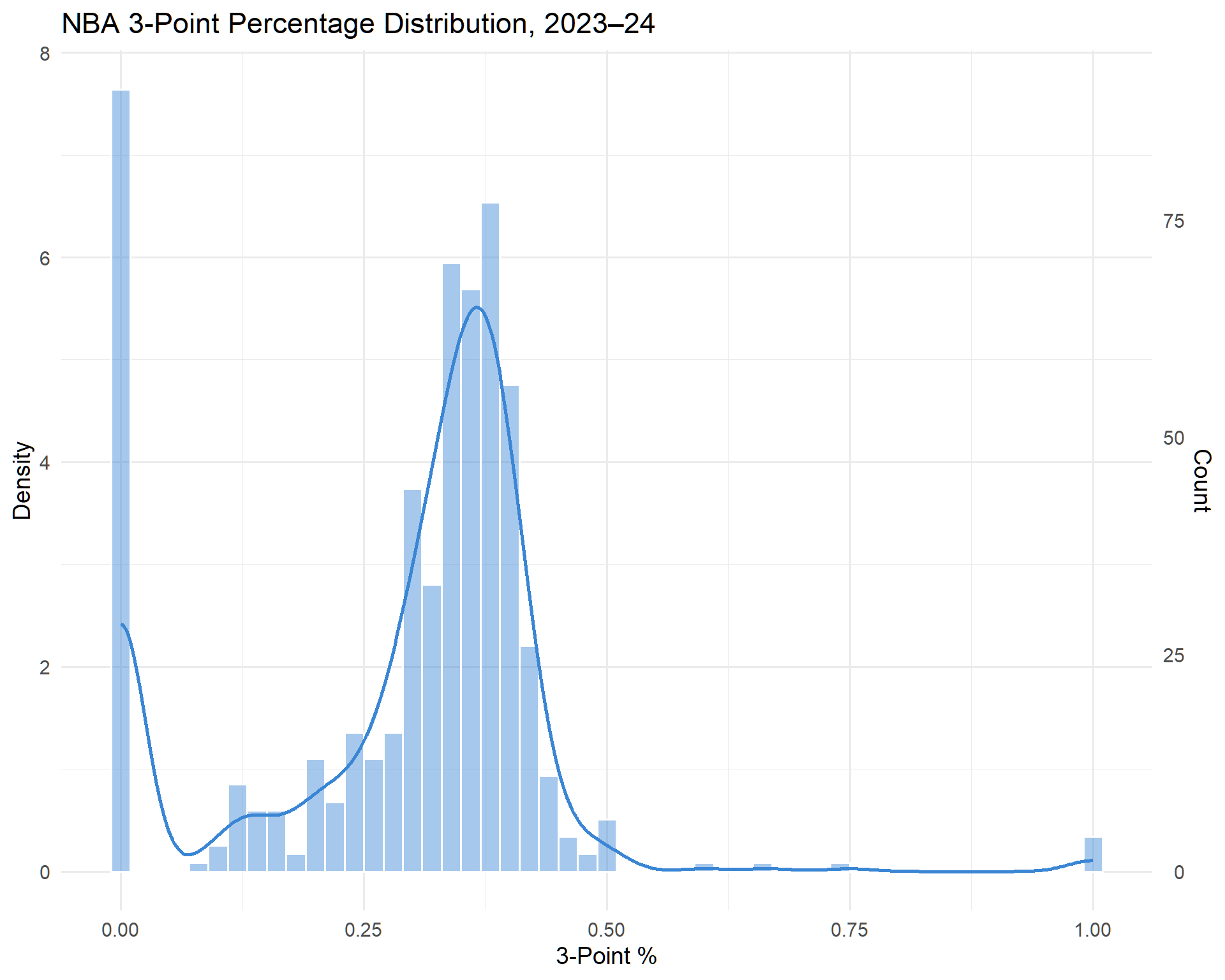
The problem with a stat like using the three_point_pct is that it treats every player's percentages as equally trustworthy. A player who shot 40% on 300 attempts and a player who shot 100% on 1 attempt are not comparable, even though the raw number for the second player looks better.
Think about it from a coin-flip perspective, flipping the coin twice in a row and get heads both times, and you'd have a 100% chance of head but it is not trustworthy. As you flip the coin continuously for many times, it will converge toward the coin's true 50% probability. Same logic applies to Kornet, what if he'd taken more attempts? As the number of attempts grows, the raw percentage becomes a much more reliable estimate of a player's true shooting ability.
This is exactly the kind of problem empirical Bayes is designed to solve: rather than trusting every player's raw percentage equally, we can build a prior from the data — an estimate of what a "typical" NBA player's three-point percentage looks like — which is usually close to the global mean.
Applying Empirical Bayes Shrinkage
To apply empirical Bayes shrinkage, we first need to specify the prior distribution using data itself. Unlike the standard Bayes approach, where prior can be obtained from previous knowledge, published literature or simply be left vague, empirical Bayes estimates prior from the current data. For this analysis, we will use the beta prior which is suitable for this context as we are modelling the rate of success. The model can be written as:
where pᵢ is player i's true three-point shooting percentage. We can estimate the beta distribution's shape using the method of moments, which uses the sample mean x̄ and variance s² of players' three-point percentages to solve for the distribution's two shape parameters:
Once we have α and β, we can apply empirical Bayes shrinkage to each player's raw percentage. Rather than trusting the observed rate alone, we combine it with the prior using the following formula:
Result
We only use players with at least 20 three-point attempts because those outliers would skew our estimate and the fitted model is shown below:
three_pts_2024_filtered = three_pts_2024 %>%
  filter(three_point_field_goals_attempted>=20)


# method-of-moments
mu = mean(three_pts_2024_filtered$three_point_pct)
var = var(three_pts_2024_filtered$three_point_pct)

alpha_mm = mu * ((mu * (1 - mu) / var) - 1)
beta_mm = alpha_mm * (1 - mu) / mu


  ggplot()+
  geom_histogram(data= three_pts_2024_filtered,aes(x= three_point_pct,y = ..density..),binwidth = binwidth,
                 color = "white", fill = "#3a86d4", alpha = 0.45)+
  geom_density(data = tibble(n = rbeta(1000,alpha_mm,beta_mm) ),aes(x=n),
               color = "#0C2340", linewidth = 1)+
  ggtitle("NBA 3-Point Percentage Distribution (attempts >=20), 2023–24") +
  scale_y_continuous(
    name = "Density",
    sec.axis = sec_axis(~ . * n * binwidth, name = "Count"))+
  labs(x="3-Point %")+
  theme_minimal(base_size = 14)
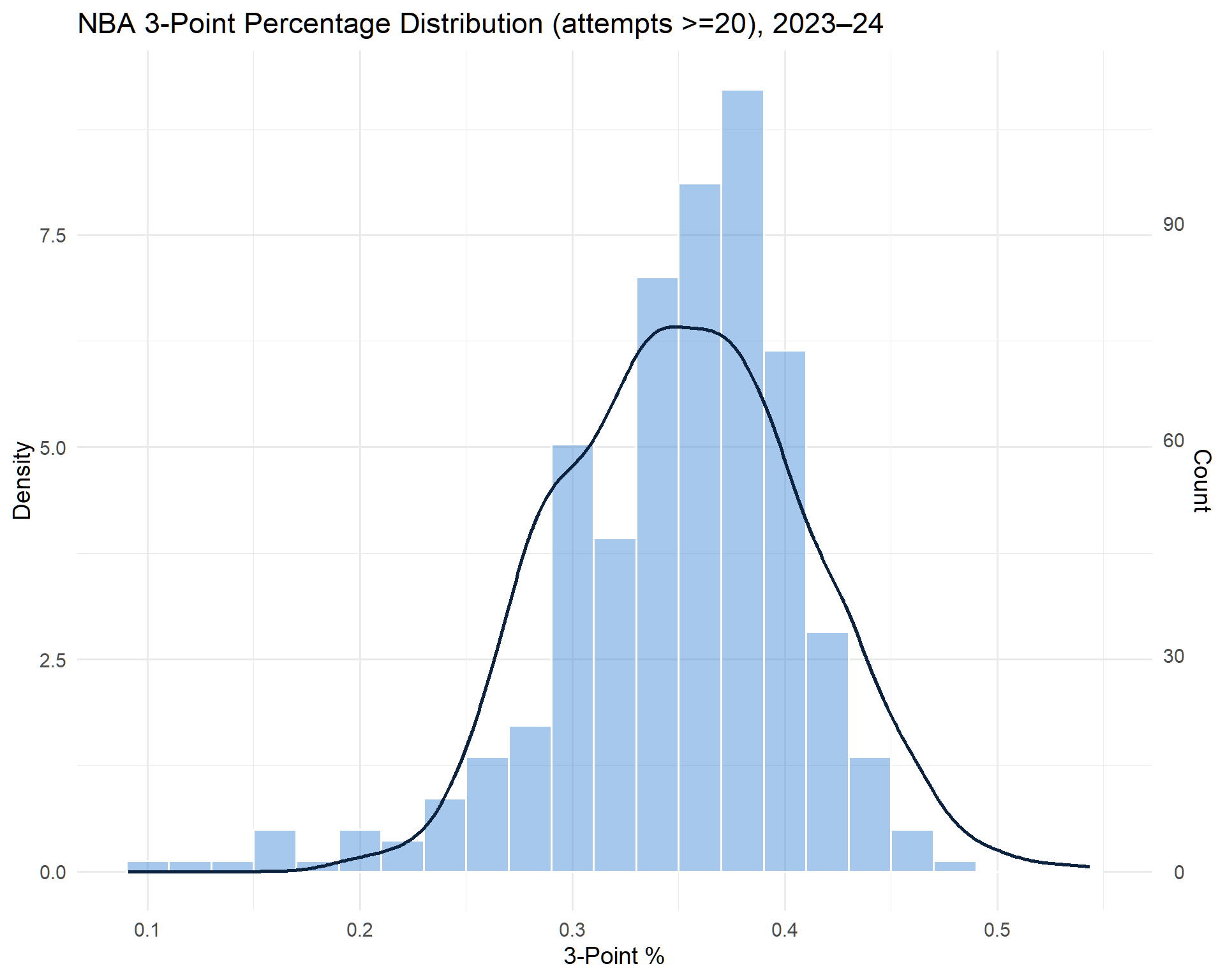
The fitted alpha is 26.4467 and beta is 45.57433, and it looks pretty decent, nicely fitted. The next step is to apply the formula to each individual player and see if it has worked out.
# Use the distribution as a prior for each NBA player estimate

three_pts_2024_filtered_eb = three_pts_2024 %>%
    mutate(alpha = alpha_mm,
           beta = beta_mm,
           eb_three_point_pct= (three_point_field_goals_made+alpha)/(three_point_field_goals_attempted+alpha+beta))

three_pts_2024_filtered_eb %>%
  dplyr::select(player=athlete_display_name,
                made = three_point_field_goals_made,
                attempted = three_point_field_goals_attempted,
                raw = three_point_pct,
                eb = eb_three_point_pct) %>%
  filter(player %in% c("Luke Kornet", "DeAndre Jordan",
                       "Stephen Curry", "Jayson Tatum")) %>%
  arrange(desc(raw))
# A tibble: 4 × 5
  player          made attempted   raw    eb
  <chr>          <int>     <int> <dbl> <dbl>
1 Luke Kornet        1         1 1     0.358
2 Stephen Curry    364       896 0.406 0.402
3 Jayson Tatum     272       756 0.360 0.359
4 DeAndre Jordan     0         0 0     0.349
Well, we can see that we have successfully applied the EB shrinkage and Kornet is no longer sitting at a ridiculous perfect 100% three-points rate. DeAndre Jordan with no attempts at all, gets pulled to the league mean, since we have no evidence to say he is anything other than average from the current data. Meanwhile, shooters like Curry and Tatum, their rates did not change much after shrinkage, it is because they have a good number of attempts and their raw percentages are already reliable estimates of their true shooting ability, so the prior has little left to correct.
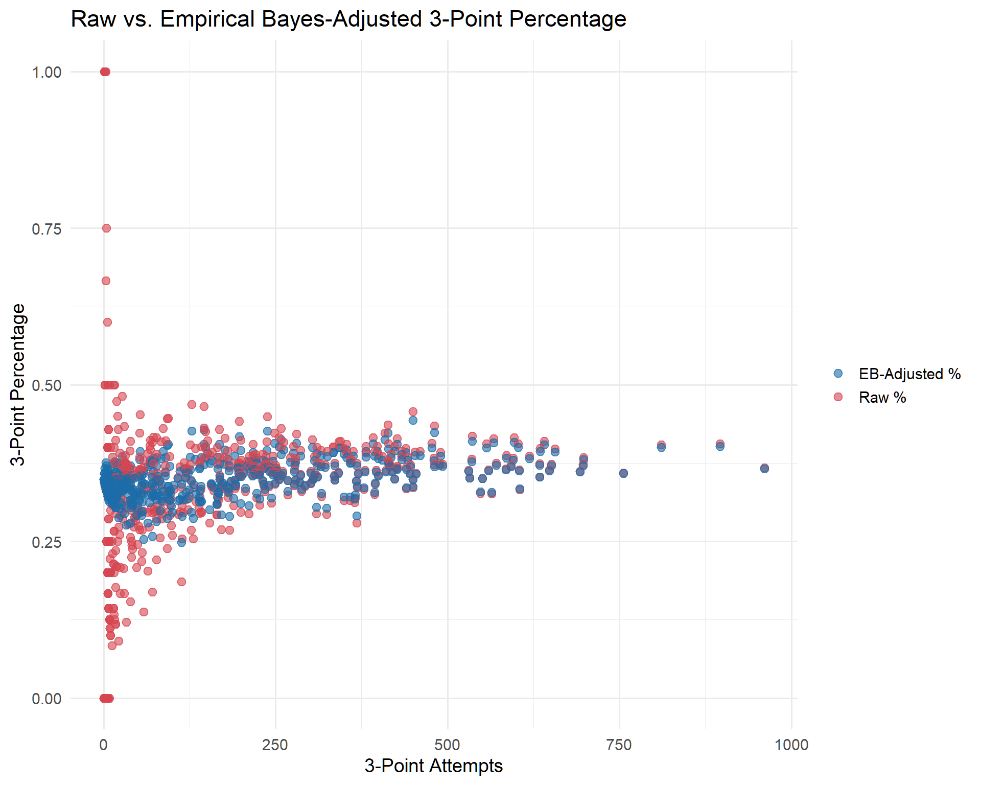
We can also observe the effect visually. The below shows the raw and empirical Bayes-adjusted 3-point percentages plotted against attempts. The funnel shape here tells the whole story: raw percentages (red) are noisy at low attempts, while EB-adjusted percentages (blue) stay close to the league average until there's enough data to trust them.
three_pts_2024_filtered_eb %>%
  pivot_longer(cols = c(three_point_pct,eb_three_point_pct),
               names_to = "type",
               values_to = "pct") %>%
  ggplot(aes(x=three_point_field_goals_attempted, y =pct,color = type))+
  geom_point(alpha=0.6,size=2.5)+
  scale_color_manual(
    values = c("three_point_pct" = "#D64550", "eb_three_point_pct" = "#1B6CA8"),
    labels = c("three_point_pct" = "Raw %", "eb_three_point_pct" = "EB-Adjusted %")
  ) +
  labs(x = "3-Point Attempts",
       y = "3-Point Percentage",
       color = NULL,
       title = "Raw vs. Empirical Bayes-Adjusted 3-Point Percentage") +
  theme_minimal(base_size = 14)
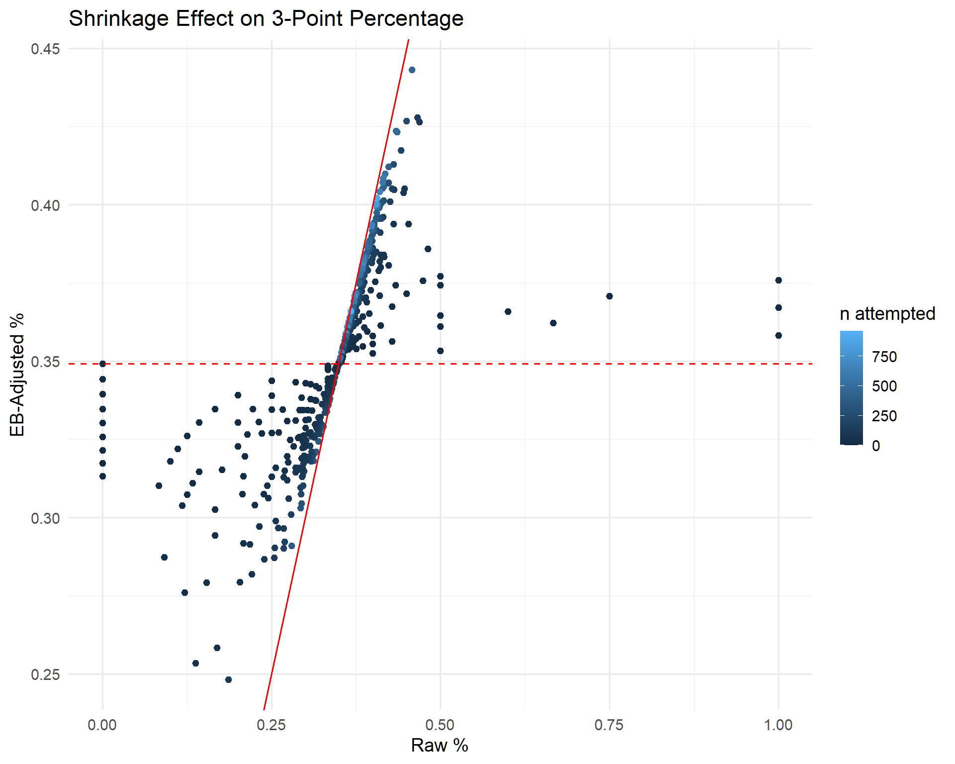
This plot below shows the shrinkage effect directly. The diagonal red line marks where raw and EB-adjusted percentages would be identical, the dashed red line marks the league-average prior. We can see the lighter blue bubbles (larger sample size) are very close to diagonal line, indicating that the shrinkage effect is minimal to these observations. Points far from the diagonal which are coloured in darker blue mostly are low-attempt players. They demonstrate the biggest pull toward the prior.
three_pts_2024_filtered_eb %>%
  ggplot(aes(x=three_point_pct, y =eb_three_point_pct))+
  geom_point(aes(color = three_point_field_goals_attempted))+
  geom_abline(intercept = 0, slope = 1, color = "red")+
  geom_hline(yintercept = alpha_mm / (alpha_mm + beta_mm), color = "red", linetype = "dashed")+
  labs(x = "Raw %",
       y = "EB-Adjusted %",
       color = "n attempted",
       title = "Shrinkage Effect on 3-Point Percentage") +
  theme_minimal(base_size = 14)
Limitation
Although EB shrinkage reduces the influence of extreme three-point percentages caused by small sample sizes, the resulting estimates are not always substantively convincing. Again, Luke Kornet and DeAndre Jordan are both shrunk towards the league mean of around 34.9% which itself is questionable. These centre players who realistically are not trained for shooting. And when Tatum, an All-Star wing, ends up shooting about only 1 percentage point higher than them, something clearly seems off.
This issue is that we assume all the players are drawn from the same underlying distribution of three-point shooting ability. Imposing league-wide Beta prior may introduce excessive pooling across different types of players. The model accounts for differences in the number of attempts, but it does not account for relevant player characteristics such as position, offensive role or historical shooting performance. A better approach could be using position-specific priors or hierarchical Empirical Bayes model. In this way, EB shrinkage may work better in shrinking players towards the average of a more comparable group.
Conclusion
We demonstrated the simple application of empirical Bayes shrinkage to improve inference of small sample sizes using the NBA three-point shooting percentages. Results show that the shrinkage does work to reduce the influence of extreme percentages.
However, using a league mean is likely too simple because it assumes all players are drawn from the same underlying distribution of three-point shooting ability. In fact, players differ substantially in position, offensive role, shot selection and historical performance. Therefore, shrinking every player towards the same mean may produce estimates that are still unrealistic.