What Determines Hair Loss? A Bayesian Logistic Regression Analysis

Background

Hair loss is a common health and appearance concern. It can be associated with age, genetics, hormonal changes, medical conditions, medications, nutritional deficiencies, stress and lifestyle factors.

This article converts a completed Quarto analysis into an MDX blog post. The goal is to practise Bayesian logistic regression and model comparison, not to make clinical claims or build a production diagnostic tool.

The data

Each row in the dataset represents one survey participant. To avoid exposing raw records, this post describes the analysis workflow and model summaries without reproducing the source dataset.

The main variables include:

• Genetics: family history of baldness
• Hormonal Changes: whether the person experienced hormonal changes
• Medical Conditions: medical history that may be associated with hair loss
• Medications & Treatments: treatment history that may be associated with hair loss
• Nutritional Deficiencies: listed deficiencies such as iron or vitamin D deficiency
• Stress: stress level
• Age: age of the participant
• Poor Hair Care Habits: whether poor hair care habits were reported
• Environmental Factors: whether environmental exposures were reported
• Smoking: smoking status
• Weight Loss: whether significant weight loss was reported
• Hair Loss: binary outcome indicating presence or absence of hair loss

suppressPackageStartupMessages({
  library(bayesrules)
  library(rstanarm)
  library(bayesplot)
  library(tidyverse)
  library(tidybayes)
  library(broom.mixed)
  library(readr)
  library(data.table)
  library(janitor)
})

data = read.csv(file = "hair_loss_data.csv")
str(data)

missing_values = sapply(data, function(x) sum(is.na(x)))
missing_values

The dataset contains one row per participant.
No missing values were detected by NA checks, but some character fields contain "No Data".

Data cleaning

Most fields are categorical or binary, so they are converted into factors. The outcome is recoded as a factor with No and Yes levels. Rows containing "No Data" are removed for simplicity, and duplicate identifiers are excluded.

data$Genetics = factor(data$Genetics, levels = c("No", "Yes"))
data$Hormonal.Changes = factor(data$Hormonal.Changes, levels = c("No", "Yes"))
data$Medical.Conditions = factor(data$Medical.Conditions)
data$Medications...Treatments = factor(data$Medications...Treatments)
data$Nutritional.Deficiencies = factor(data$Nutritional.Deficiencies)
data$Stress = factor(data$Stress)
data$Age = as.numeric(data$Age)
data$Poor.Hair.Care.Habits = factor(data$Poor.Hair.Care.Habits)
data$Environmental.Factors = factor(data$Environmental.Factors)
data$Smoking = factor(data$Smoking, levels = c("No", "Yes"))
data$Weight.Loss = factor(data$Weight.Loss, levels = c("No", "Yes"))
data$Hair.Loss = factor(
  ifelse(data$Hair.Loss == 1, "Yes", "No"),
  levels = c("No", "Yes")
)

data = data %>%
  filter(if_all(everything(), ~ . != "No Data"))

data %>%
  group_by(Id) %>%
  filter(n() > 1)

data = data %>%
  mutate(Id = as.character(Id)) %>%
  filter(Id != "157627" & Id != "110171")

Rows with "No Data" were removed.
Two duplicated participant identifiers were excluded from the modelling data.

Specifying priors

The outcome is binary, so the models use Bayesian logistic regression. The intercept prior is specified on the log-odds scale.

Because the analysis is not based on domain expertise, the intercept prior is set using a broad expected range for hair loss prevalence. A plausible average probability range from about 16 percent to 50 percent corresponds roughly to log-odds from -1.66 to 0.

That gives a midpoint near -0.83, so the model uses:

prior_intercept = normal(-0.8, 0.4)

For other coefficients, weakly informative priors are used:

prior = normal(0, 2.5, autoscale = TRUE)

This keeps the model regularised while still allowing associations to be learned from the data.

Model 1: age, genetics and hormonal changes

The first model is intentionally simple. It includes age, genetics and hormonal changes.

model_1 = stan_glm(
  Hair.Loss ~ Age + Genetics + Hormonal.Changes,
  data = data,
  family = binomial,
  prior_intercept = normal(-0.8, 0.4),
  prior = normal(0, 2.5, autoscale = TRUE),
  chains = 4,
  iter = 5000 * 2,
  seed = 87453804
)

Posterior diagnostics are checked using trace plots, density overlays and autocorrelation plots.

mcmc_trace(model_1)
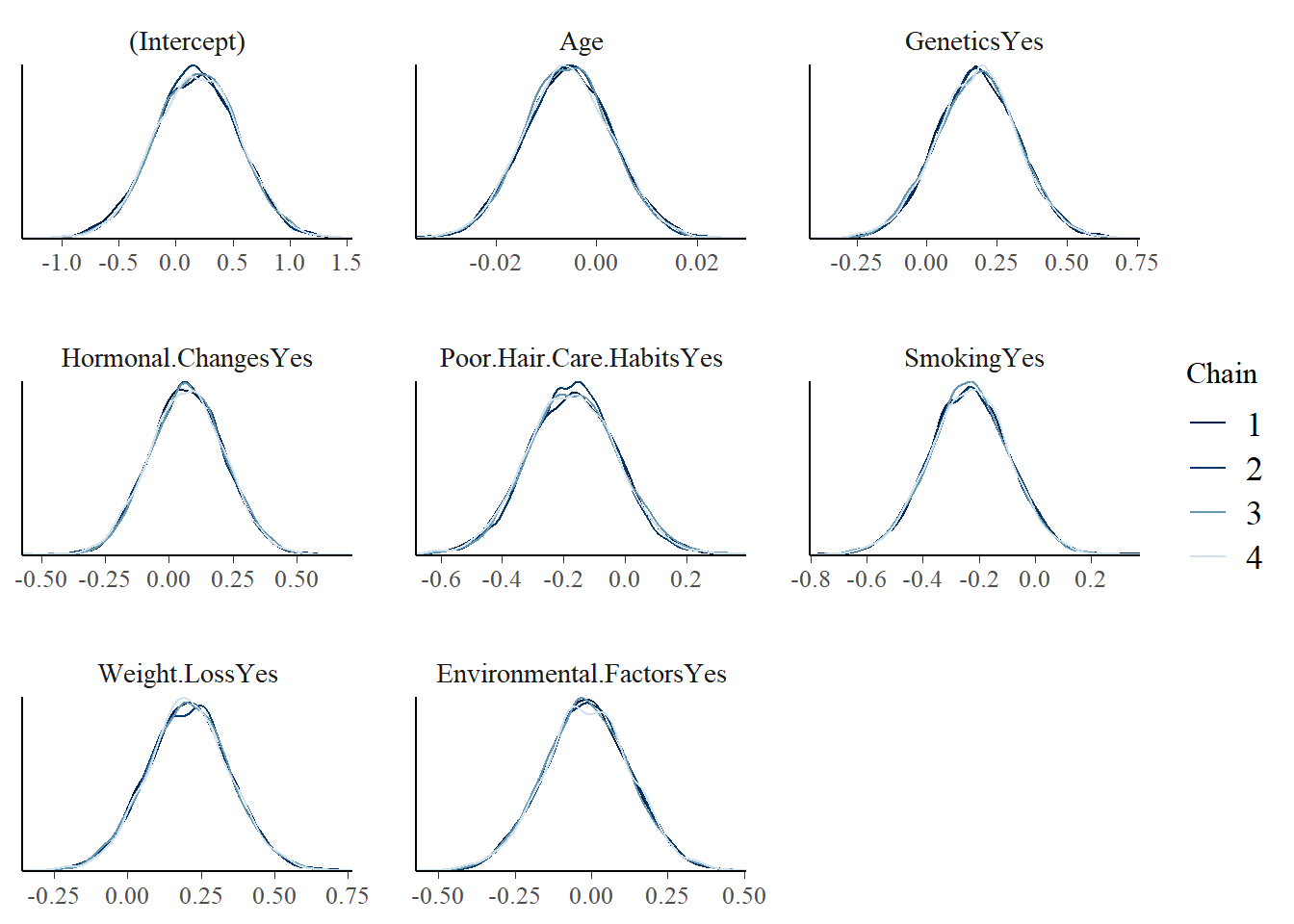
mcmc_dens_overlay(model_1)
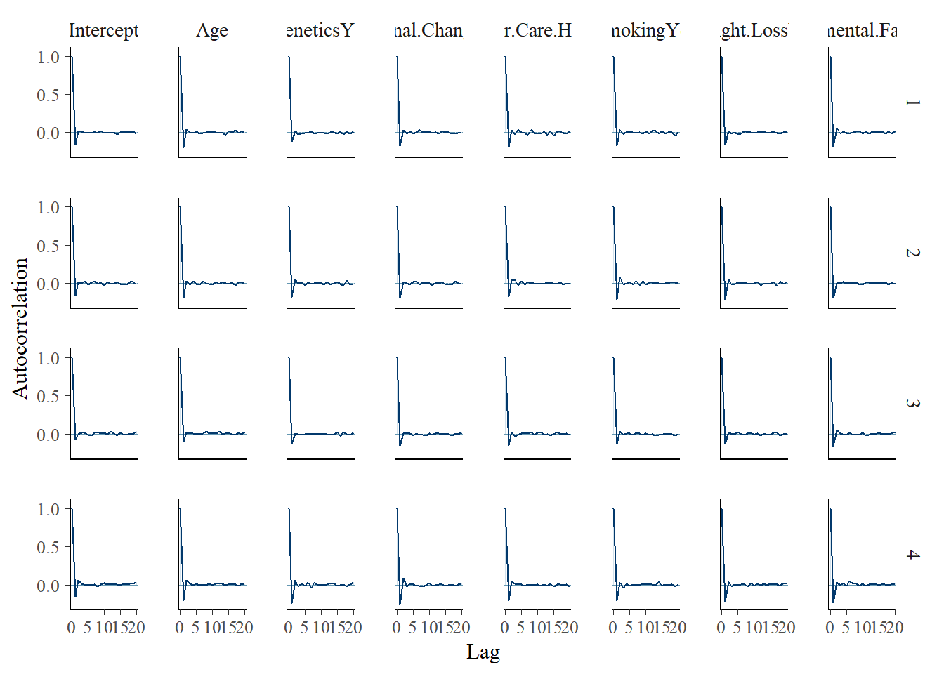
mcmc_acf(model_1)

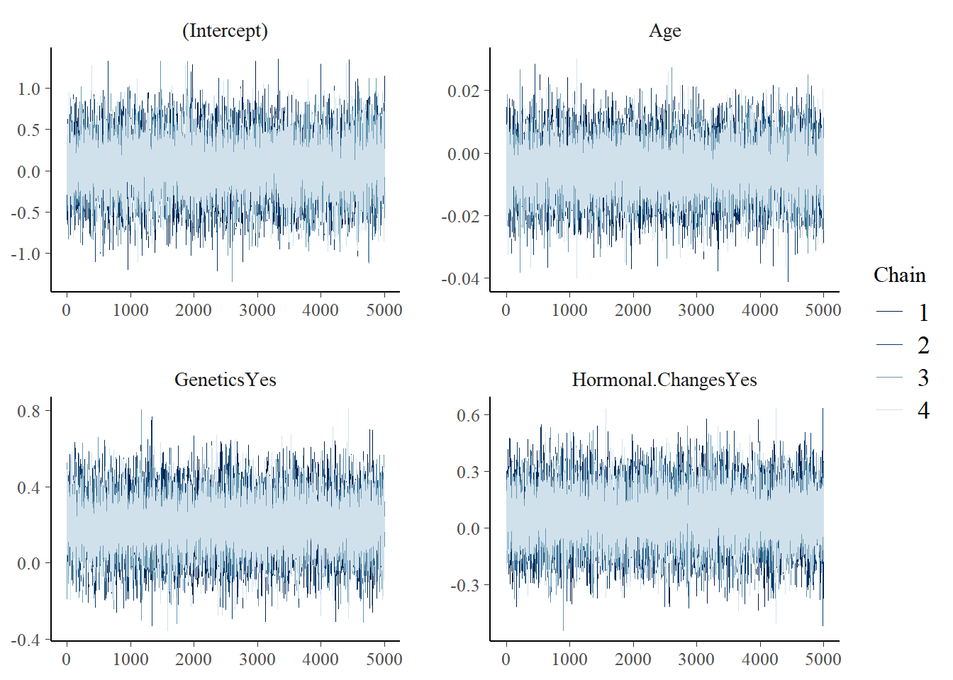
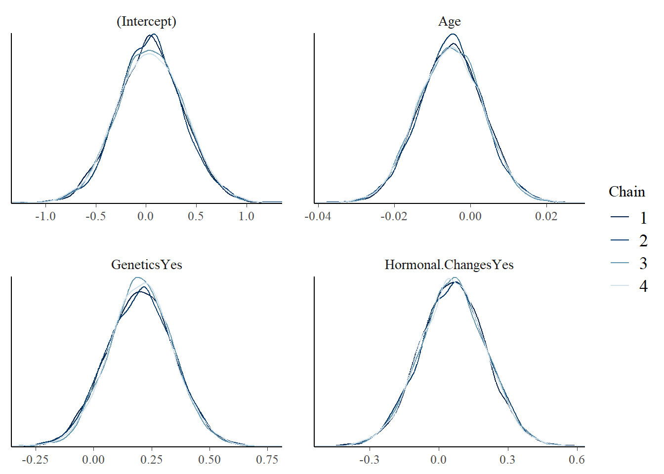
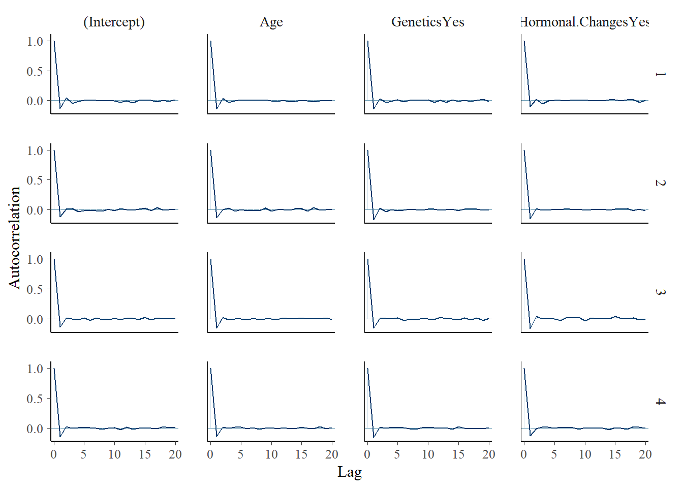
The diagnostics suggest the simulation is stable enough for this practice analysis.

tidy(
  model_1,
  effects = "fixed",
  conf.int = TRUE,
  conf.level = 0.8
)

Model 1 summary:
- Age: 80% credible interval overlaps 0 on the log-odds scale.
- Hormonal changes: 80% credible interval overlaps 0.
- Genetics: positive association at the 80% credible interval in this simple model.

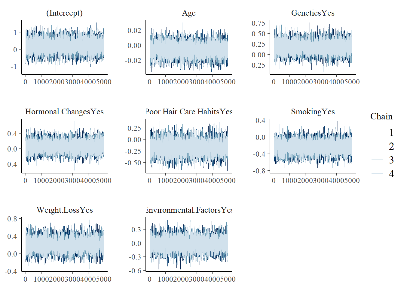
Model 2: adding lifestyle and environmental factors

The second model adds poor hair care habits, smoking, weight loss and environmental factors.

model_2 = stan_glm(
  Hair.Loss ~ Age + Genetics + Hormonal.Changes +
    Poor.Hair.Care.Habits + Smoking + Weight.Loss +
    Environmental.Factors,
  data = data,
  family = binomial,
  prior_intercept = normal(-0.8, 0.4),
  prior = normal(0, 2.5, autoscale = TRUE),
  chains = 4,
  iter = 5000 * 2,
  seed = 87453804
)

mcmc_trace(model_2)
mcmc_dens_overlay(model_2)
mcmc_acf(model_2)

tidy(
  model_2,
  effects = "fixed",
  conf.int = TRUE,
  conf.level = 0.8
)

Model 2 summary:
- Most 80% credible intervals overlap 0 on the log-odds scale.
- Genetics remains positively associated with hair loss.
- Weight loss also appears as a potentially meaningful predictor.

Model 3: adding medical conditions, treatments and stress

The third model includes the remaining predictors: medical conditions, medications/treatments and stress. Reference levels are set before fitting the model.

data[["Medical.Conditions"]] = relevel(
  factor(data[["Medical.Conditions"]]),
  ref = "Eczema"
)

data[["Medications...Treatments"]] = relevel(
  factor(data[["Medications...Treatments"]]),
  ref = "Antibiotics"
)

data[["Stress"]] = relevel(
  factor(data[["Stress"]]),
  ref = "Low"
)

model_3 = stan_glm(
  Hair.Loss ~ Age + Genetics + Hormonal.Changes +
    Poor.Hair.Care.Habits + Smoking + Weight.Loss +
    Environmental.Factors + Medical.Conditions +
    Medications...Treatments + Stress,
  data = data,
  family = binomial,
  prior_intercept = normal(-0.8, 0.4),
  prior = normal(0, 2.5, autoscale = TRUE),
  chains = 4,
  iter = 5000 * 2,
  seed = 87453804
)

tidy(
  model_3,
  effects = "fixed",
  conf.int = TRUE,
  conf.level = 0.8
)

Model 3 summary:
- Genetics no longer clearly separates from 0 after controlling for medical conditions, treatments and stress.
- Weight loss remains a potentially meaningful predictor.
- Some medical condition categories, especially alopecia areata, appear important at the 80% credible interval.

This suggests that genetics may not add much once medical conditions, treatments and stress are included. It does not prove genetics is irrelevant; it simply shows how the association changes under a larger adjustment set.

Model 4: a reduced model

The fourth model keeps predictors that appeared more informative in previous models.

model_4 = stan_glm(
  Hair.Loss ~ Genetics + Weight.Loss + Medical.Conditions,
  data = data,
  family = binomial,
  prior_intercept = normal(-0.8, 0.4),
  prior = normal(0, 2.5, autoscale = TRUE),
  chains = 4,
  iter = 5000 * 2,
  seed = 87453804
)

tidy(
  model_4,
  effects = "fixed",
  conf.int = TRUE,
  conf.level = 0.8
)

Model 4 is a simpler candidate model using genetics, weight loss and medical conditions.
It is easier to interpret, but predictive performance still needs to be checked.

How wrong is the model?

Posterior predictive checks can show whether simulated data from the model resemble the observed outcome. Here, Model 1 is used as an example. For each posterior simulated dataset, the proportion of participants with hair loss is calculated.

proportion_hairloss_1 = function(x) {
  mean(x == 1)
}

pp_check(
  model_1,
  nreps = 100,
  plotfun = "stat",
  stat = "proportion_hairloss_1"
)

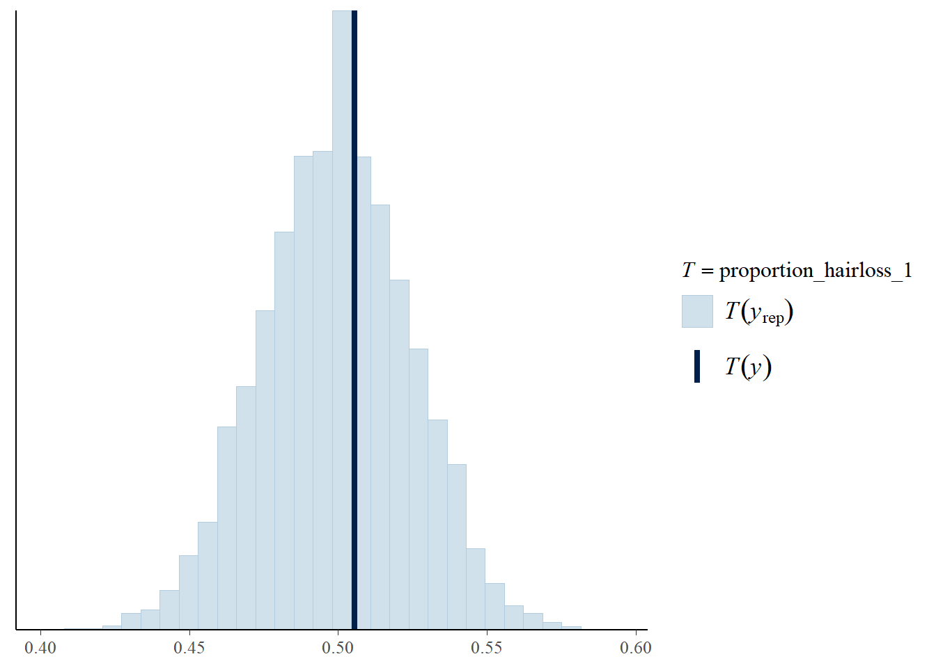
Most posterior simulated datasets show a hair loss rate near the observed rate, around 50 percent.

How accurate is the model?

Classification performance is assessed using posterior predictions and a 0.5 probability cutoff.

hair_loss_pred_1 = posterior_predict(model_1, newdata = data)

hair_loss_classification = data %>%
  mutate(
    hairloss_prob = colMeans(hair_loss_pred_1),
    hairloss_class = as.numeric(hairloss_prob >= 0.5)
  ) %>%
  tabyl(Hair.Loss, hairloss_class) %>%
  adorn_totals(c("row", "col"))

hair_loss_classification

classification_summary(
  model = model_1,
  data = data,
  cutoff = 0.5
)$accuracy_rates

Overall accuracy: 0.532

The model correctly classified 431 of 809 cases.
This is only slightly better than random guessing for a balanced binary outcome.

Cross-validation

Five-fold cross-validation is used to compare classification accuracy across the four models.

set.seed(883548)

cv_accuracy_1 = classification_summary_cv(
  model = model_1,
  data = data,
  cutoff = 0.5,
  k = 5
)

cv_accuracy_2 = classification_summary_cv(
  model = model_2,
  data = data,
  cutoff = 0.5,
  k = 5
)

cv_accuracy_3 = classification_summary_cv(
  model = model_3,
  data = data,
  cutoff = 0.5,
  k = 5
)

cv_accuracy_4 = classification_summary_cv(
  model = model_4,
  data = data,
  cutoff = 0.5,
  k = 5
)

cv_accuracy_1$cv
cv_accuracy_2$cv
cv_accuracy_3$cv
cv_accuracy_4$cv

Cross-validation summary:
Model 1 has the strongest cross-validated classification accuracy among the four candidates.
None of the models performs especially well overall.

Summary

The Bayesian logistic regression models explored whether age, genetics, hormonal changes, lifestyle factors and medical conditions were associated with hair loss in the survey data.

The results show that some predictors, such as genetics, weight loss and specific medical condition categories, may be informative in some model specifications. However, the overall classification accuracy is low, and the best model is only modestly better than random guessing.

This analysis should therefore be read as a practice exercise in Bayesian logistic regression rather than a reliable predictive model. The weak predictive performance may indicate that the available variables do not capture enough of the underlying structure, or that a simple logistic regression model is not flexible enough for this dataset.