Bayesian Linear Regression Analysis of Health Insurance Costs

Background

This post converts a completed Quarto analysis into an MDX article for the portfolio. The analysis uses a public health insurance cost dataset to practise Bayesian linear regression with rstanarm, focusing on model specification, posterior diagnostics and model comparison.

The original motivation came from working through machine learning examples in R. Some teaching datasets are not always easy to access in their book-specific cleaned form, so this example uses a freely available health insurance dataset instead. The goal is not to produce a deployable insurance pricing model, but to work through a clear Bayesian regression workflow.

The data

The dataset contains individual-level insurance records. To avoid exposing raw records, this article describes the structure and modelling workflow rather than reproducing the dataset itself.

Key columns include:

• age: age of the primary beneficiary
• sex: beneficiary sex
• bmi: body mass index
• children: number of covered dependants
• smoker: smoking status
• region: residential region in the United States
• charges: individual medical costs billed by health insurance

suppressPackageStartupMessages({
  library(bayesrules)
  library(rstanarm)
  library(bayesplot)
  library(tidyverse)
  library(tidybayes)
  library(broom.mixed)
  library(readr)
  library(data.table)
  library(janitor)
})

data = read.csv(file = "insurance.csv")
str(data)

'data.frame': 1338 obs. of 7 variables:
 $ age     : int
 $ sex     : chr
 $ bmi     : num
 $ children: int
 $ smoker  : chr
 $ region  : chr
 $ charges : num

Data cleaning

The cleaning step converts categorical variables into factors, checks for missing values and removes duplicate rows. The raw dataset is not included in this post.

summary(data)

data$sex = factor(data$sex)
data$children = factor(data$children)
data$age = as.numeric(data$age)
data$smoker = factor(data$smoker)
data$region = factor(data$region)

which(is.na(data))

data %>%
  group_by_all() %>%
  summarise(count = n()) %>%
  filter(count > 1)

data = data %>% distinct()

Missing values: none detected
Duplicate rows: one duplicated record identified and removed
Rows after cleaning: 1337

Visualisation

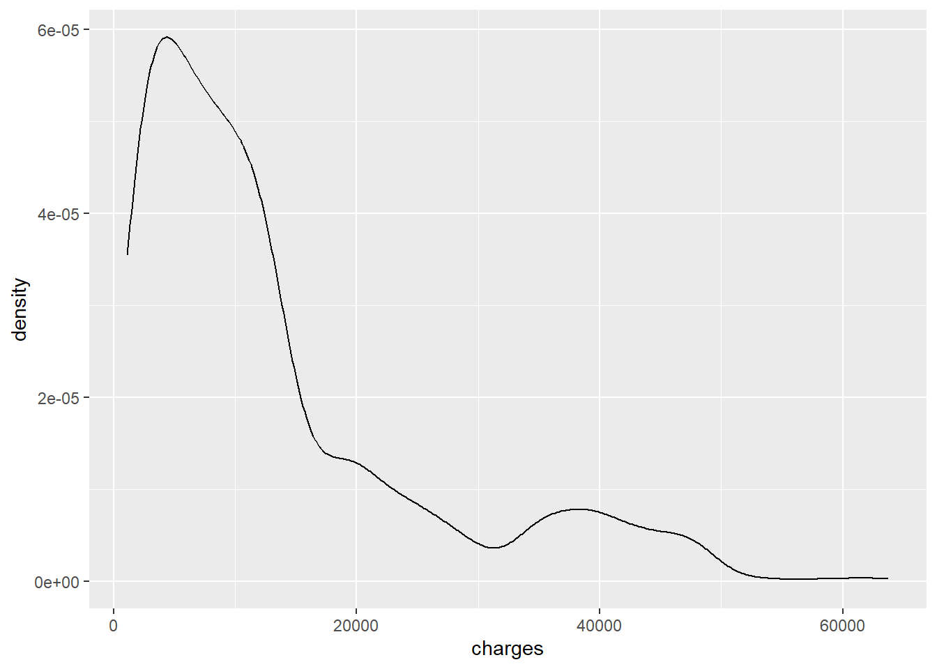
The initial visualisations show that insurance charges are heavily right-skewed. For modelling, the outcome is therefore transformed using log(charges).

ggplot(data, aes(charges)) +
  geom_density()

ggplot(data, aes(x = log(charges), fill = smoker)) +
  geom_density()

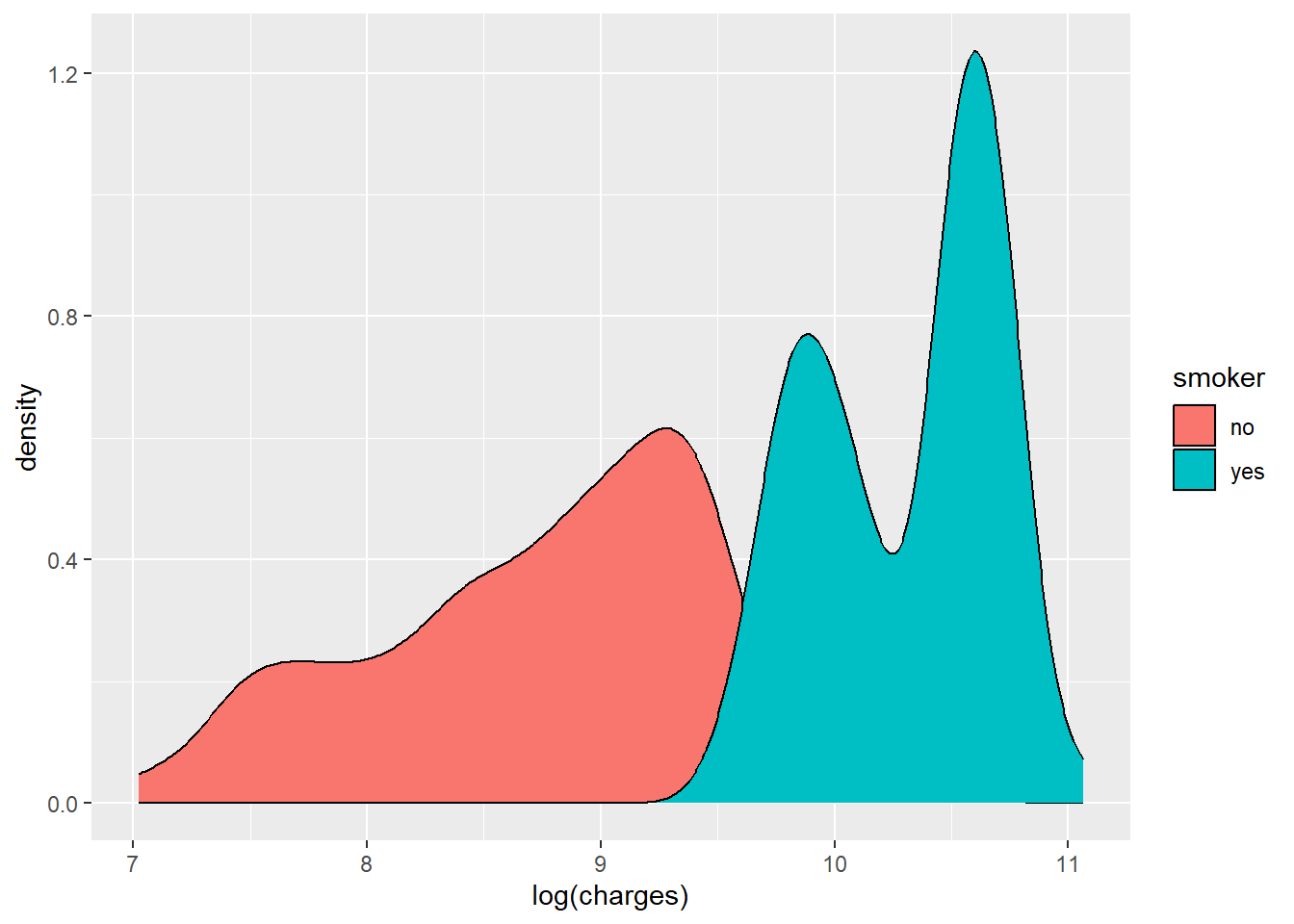
The log-transformed outcome shows clearer structure, including distinct grouping by smoking status.

ggplot(data, aes(x = age, y = log(charges), colour = smoker)) +
  geom_point()

ggplot(data, aes(x = bmi, y = log(charges), colour = smoker)) +
  geom_point()

ggplot(data, aes(x = smoker, y = log(charges))) +
  geom_boxplot()

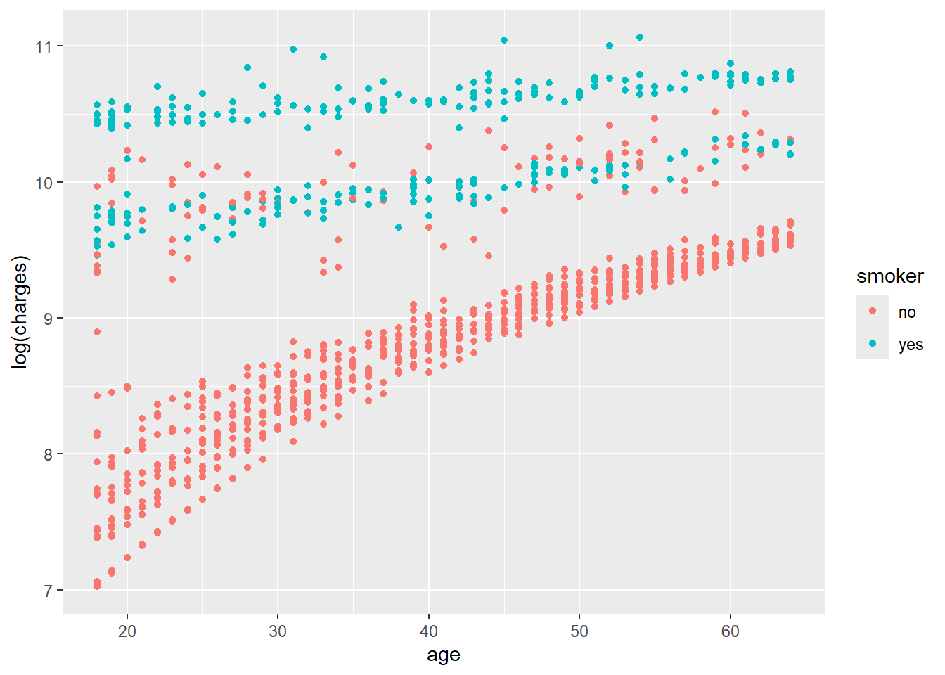
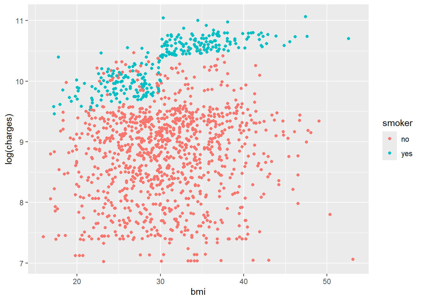
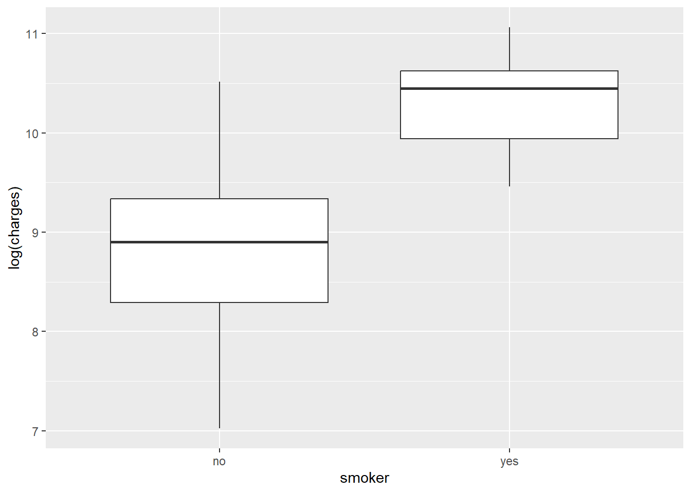
The density plots suggest clustered groups, particularly among smokers. The dataset does not contain variables that explicitly identify these clusters, which is an important limitation for a simple regression model.

Specifying priors

The response variable is log(charges), so priors need to be specified on the log scale. Because the data refer to insurance charges in the United States, the intercept prior is centred around a plausible annual cost on the log scale.

The model uses:

• a normal prior for the intercept
• weakly informative normal priors for coefficients
• an exponential prior for the residual standard deviation

This keeps the model regularised without forcing overly strong assumptions.

Simulating the posterior

Model 1 uses three predictors: smoking status, BMI and age.

data[["smoker"]] = relevel(factor(data[["smoker"]]), ref = "no")
data = data %>% mutate(log_charges = log(charges))

model_1 = stan_glm(
  formula = log_charges ~ smoker + bmi + age,
  data = data,
  family = gaussian,
  prior_intercept = normal(8.5, 0.25),
  prior = normal(0, 2.5, autoscale = TRUE),
  prior_aux = exponential(1, autoscale = TRUE),
  chains = 4,
  iter = 5000 * 2,
  seed = 87453804
)

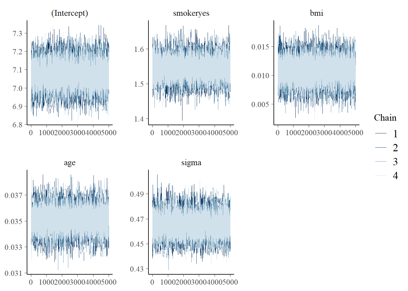
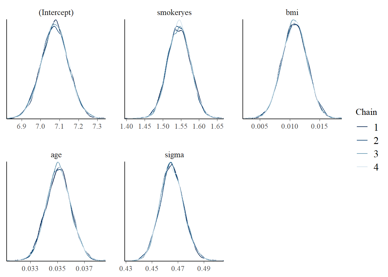
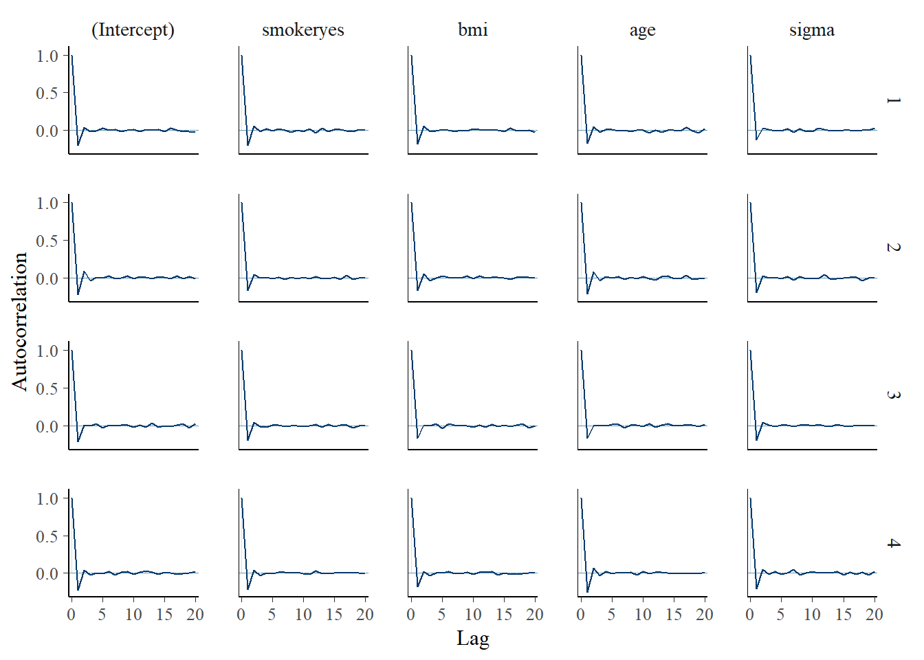
Posterior diagnostics are used to check whether the simulation appears stable.

mcmc_trace(model_1)
mcmc_dens_overlay(model_1)
mcmc_acf(model_1)

Interpreting the posterior

The fixed effects can be summarised with credible intervals.

tidy(
  model_1,
  effects = "fixed",
  conf.int = TRUE,
  conf.level = 0.8
)

term         estimate  conf.low  conf.high
(Intercept)  7.00      6.88      7.12
smokeryes    1.54      1.50      1.58
bmi          0.01      0.008     0.013
age          0.03      0.030     0.034

In this model, BMI has a small positive association with log insurance charges. A one-unit increase in BMI is associated with an approximate 1 percent increase in expected charges, holding the other variables constant.

The smoking coefficient is much larger. On the log scale, the estimate suggests that smokers have substantially higher expected charges than non-smokers, after adjusting for BMI and age.

How wrong is the model?

Posterior predictive checks compare simulated data from the model with the observed data. Here, Model 1 captures the broad range of log charges, but it does not fully reproduce the multi-peaked pattern seen in the observed distribution.

pp_check(model_1, nreps = 100) +
  xlab("log(charges)")

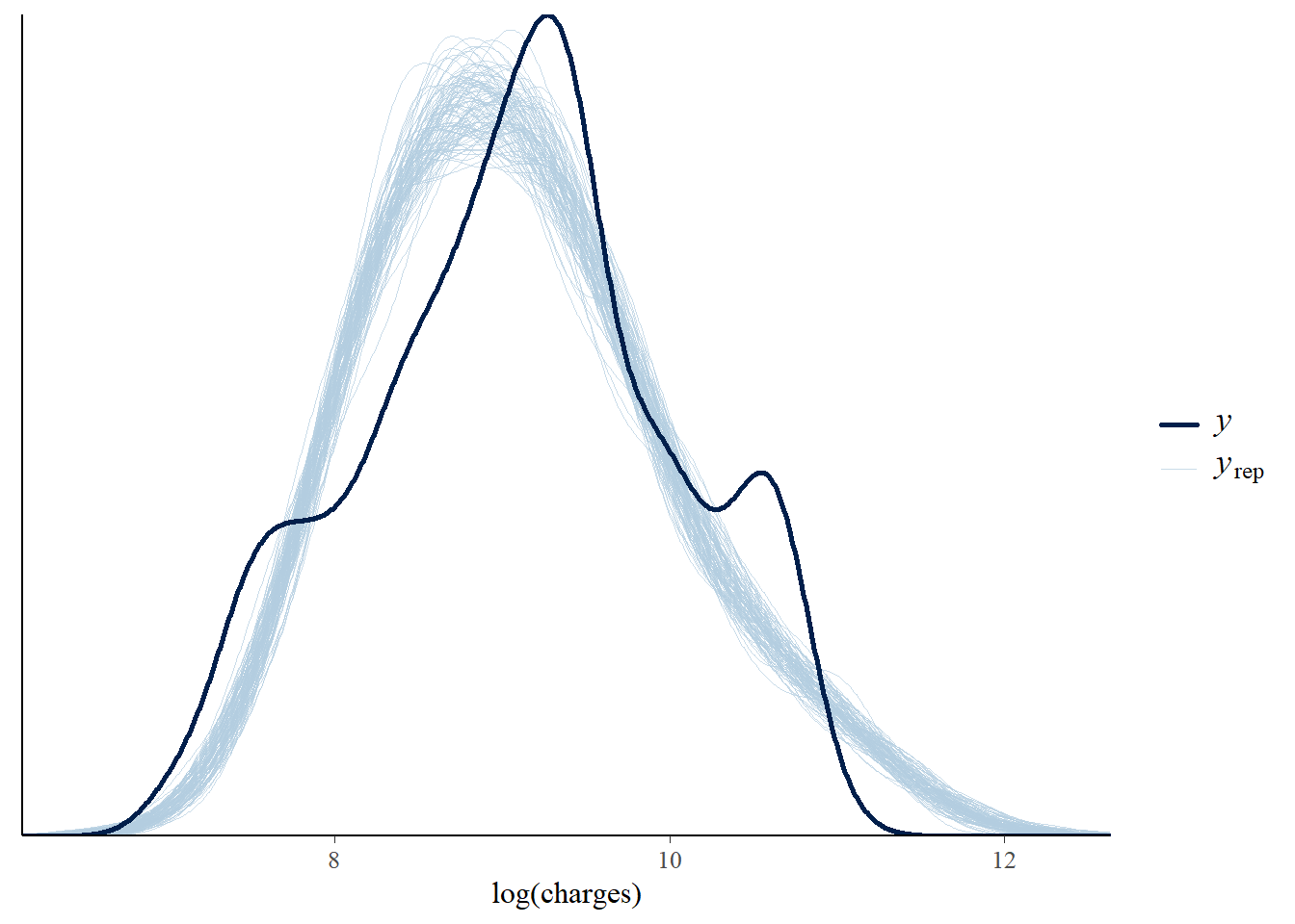
This does not mean the model is useless. It means that a simple Gaussian linear model is not rich enough to explain all structure in the data. More informative predictors, interactions or a different modelling approach may be needed.

Model evaluation and comparison

Model 2 adds all available predictors from the dataset: smoking status, BMI, age, number of children and region.

data[["children"]] = relevel(factor(data[["children"]]), ref = "0")

model_2 = stan_glm(
  formula = log_charges ~ smoker + bmi + age + children + region,
  data = data,
  family = gaussian,
  prior_intercept = normal(8.5, 0.25),
  prior = normal(0, 2.5, autoscale = TRUE),
  prior_aux = exponential(1, autoscale = TRUE),
  chains = 4,
  iter = 5000 * 2,
  seed = 87453804
)

A 10-fold cross-validation comparison is used to compare prediction error.

set.seed(84025797)

cv_model_1 = prediction_summary_cv(model = model_1, data = data, k = 10)
cv_model_2 = prediction_summary_cv(model = model_2, data = data, k = 10)

rbind(
  cv_model_1$cv %>% mutate(model = "1") %>% select(model, everything()),
  cv_model_2$cv %>% mutate(model = "2") %>% select(model, everything())
)

model  mae      mae_scaled
1      higher   higher
2      lower    lower

Model 2 shows slightly better predictive performance in cross-validation. However, the improvement is modest relative to the increase in model complexity.

Expected log predictive density gives another view of out-of-sample predictive performance while accounting for uncertainty.

loo_1 = loo(model_1)
loo_2 = loo(model_2)

c(
  loo_1$estimates[1],
  loo_2$estimates[1]
)

loo_compare(loo_1, loo_2)

Model 2 has the better expected log predictive density.
The ELPD comparison suggests a meaningful improvement in out-of-sample prediction.

Cross-validation alone suggested only a small improvement, but the ELPD comparison gives stronger support for Model 2. In this case, the additional predictors appear to improve predictive performance enough to justify the added complexity.

Conclusion

This analysis used Bayesian linear regression to model log health insurance charges with predictors such as age, smoking status, BMI, children and region. The models capture some broad patterns in the data, especially the strong difference between smokers and non-smokers.

The posterior predictive check also highlights a limitation: simple linear regression does not reproduce the multi-peaked distribution of insurance charges. That is expected given the limited set of predictors and the structure visible in the exploratory plots.

As a practice exercise in Bayesian regression, the analysis is useful for demonstrating prior specification, posterior simulation, diagnostics and model comparison. For a production prediction task, the next step would be to test richer model structures and evaluate whether additional predictors can explain the remaining clusters in the outcome distribution.